Source

Naive Bayes is a supervised machine learning algorithm base on Bayes Theorem.

Naive because it assumes all of the predictor variables to be completely independent of each other.

Bayes Rule:

P(A|B) = \frac{P(B|A)P(A)}{P(B}

P(A|B): Conditional probability of event A occuring, given event B
P(A): Probability of event A occuring
P(B): Probability of event B occuring
P(B|A): Conditional probability of event B occuring, given event A

In Naive Bayes, there are multiple predictor variables and more than 1 output class.

The objective of a Naive Bayes algorithm is to measure the conditional probability of an event with a feature vector

Problem Statement:

Predict employee attrition

Code

data("attrition")
attrition <- attrition %>%
                mutate(JobLevel = factor(JobLevel),
                       StockOptionLevel = factor(StockOptionLevel),
                       TrainingTimesLastYear = factor(TrainingTimesLastYear))

Create training (70%) and test (30%) sets and utilize reproducibility.

Code

set.seed(123)
split <- initial_split(data = attrition, prop = 0.7, strata = "Attrition")

train <- training(split)
test  <- testing(split)

Distribution of Attrition rates across train and test sets.

Code

prop.table(table(train$Attrition))


       No       Yes 
0.8394942 0.1605058

Code

prop.table(table(test$Attrition))


       No       Yes 
0.8371041 0.1628959

Notice that they are very similar.

A Naive Overview

The Naive Bayes classifier is founded on Bayesian probability, which incorporates the concept of conditional probability.

In our attrition data set, we are seeking the probability of an employee belonging to attrition class C_{k} given the predictor variables x_{1}, x_{2}, ... x_{n}

A posterior:

Posterior = \frac{Prior * Likelihood}{Evidence}

Assumption:

The Naive Bayes classifier assumes that the predictor variables are conditionally independent of each other, with no correlation.

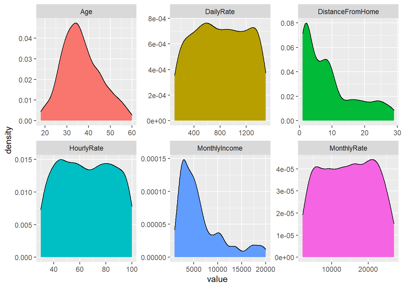
An assumption of normality is often used for continuous variables.

But you can see that normality assumption is not always held:

Code

train %>% 
  select(Age, DailyRate, DistanceFromHome, HourlyRate, MonthlyIncome, MonthlyRate) %>% 
  gather(metric, value) %>% 
  ggplot(aes(value, fill = metric)) + 
  geom_density(show.legend = FALSE) + 
  facet_wrap(~ metric, scales = "free")

Advantages and Shortcoming

The Naive Bayes classifier is simple, fast, and scales well to large n.

A major disadvantage is that it relies on the often-wrong assumption of equally important and independent features.

Implementation

We will utilize the caret package in R.

Create response and feature data

Code

features <- setdiff(names(train), "Attrition")
x <- train[, features]
y <- train$Attrition

Initialize 10-fold cross validation using caret’s trainControl function.

Code

trControl <- trainControl(method = "cv", number = 10)

Training the Naive Bayes model:

Code

nb.fit <- train(
  x = x,
  y = y,
  method = "nb",
  trControl = trControl
)

#Confusion Matrix to analyze our results:

Code

confusionMatrix(nb.fit)

Cross-Validated (10 fold) Confusion Matrix 

(entries are percentual average cell counts across resamples)
 
          Reference
Prediction   No  Yes
       No  76.8  8.2
       Yes  7.1  7.9
                            
 Accuracy (average) : 0.8473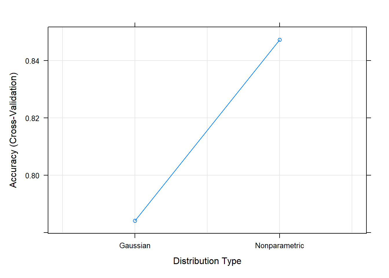

Code

plot(nb.fit)

To test the accuracy on our test data set:

Code

preds <- predict(nb.fit, newdata = test)

Code

confusionMatrix(preds, reference = test$Attrition)

Confusion Matrix and Statistics

          Reference
Prediction  No Yes
       No  329  38
       Yes  41  34
                                          
               Accuracy : 0.8213          
                 95% CI : (0.7823, 0.8559)
    No Information Rate : 0.8371          
    P-Value [Acc > NIR] : 0.8333          
                                          
                  Kappa : 0.3554          
                                          
 Mcnemar's Test P-Value : 0.8220          
                                          
            Sensitivity : 0.8892          
            Specificity : 0.4722          
         Pos Pred Value : 0.8965          
         Neg Pred Value : 0.4533          
             Prevalence : 0.8371          
         Detection Rate : 0.7443          
   Detection Prevalence : 0.8303          
      Balanced Accuracy : 0.6807          
                                          
       'Positive' Class : No